Using the AnalyzeTimeSeries Class

This class contains a set of methods to create a database of data from KPF observations, as well as methods to ingest data, query the database, print data, and made plots of various types. The script ingest_kpf_ts_db.py can be used to ingest data from the command line.

The ingested data comes from PRIMARY header extensions of L0/2D/L1/L2 files, RV and CCF header extensions in L2 files, TELEMETRY extensions in L0 files.

An elaborate set of standard time series plots can be made over intervals of days/months/years/decades spanning a date range. Plots of the number of observations of a given type (e.g., flats) over time can also be produced in standardized ways.

This code is designed to be used in several ways. First, it can be run in ‘production’ mode on a central server to regularly generate a set of plots showing the state of KPF and its data products to inform observers and DRP developers. Within the KPF team, display of these plots is through the Jump web interface. The plotting methods offer a way for KPF afficianados to quickly diagnose hardware and software issues that are evident by comparing data from different observations and to assess remedies. This work can be done using a Jupyter Notebook or with production scripts running automatically. All of the standard Quality Control (QC) and Diagnostics outputs generated by the DRP are ingested automatically. Thus, users don’t need to scrape FITS headers for this information. The databases also offer a way to package derived KPF data products (e.g., RVs and metadata) into a single file for distribution and relatively easy access for analysis.

The AnalyzeTimeSeries class provides a front end to database methods inthe TSDB class. Under the hood, TSDB can use either a portable SQLite3 database stored in a file or a Postgresql database configured on a server. Distinctions between the SQLite3 and Postgresql implementations are discusssed on the related page titled “Database Details - SQLite and PostgreSQL”.

This tutorial describes the basics of data ingestion, querying and display of the database, and making standardized time series plots and histograms of the number of observations vs. time. For additional details about capabilities, the user is encouraged to read the code in KPF-Pipeline/database/modules/src/utils/tsdb.py and KPF-Pipeline/modules/quick_look/src/analyze_time_series.py.

To use AnalyzeTimeSeries methods, start by importing packages.

[1]:

from modules.quicklook.src.analyze_time_series import AnalyzeTimeSeries
import pandas as pd
import matplotlib.pyplot as plt
import os
import numpy as np
import time
import subprocess
import matplotlib.dates as mdates
from datetime import datetime
from astropy.table import Table
%matplotlib inline

Database Ingestion

The AnalyzeTimeSeries class is initiated as shown below. This example uses a SQLite3 database, which is fresh because the file kpf_ts.db didn’t exist. When running the database in another environment, the user may want to specify a different db_path.

[2]:

db_path = 'kpf_ts.db' # name of database file
myTS = AnalyzeTimeSeries(db_path=db_path)

INFO: Starting AnalyzeTimeSeries
INFO: Starting KPF_TSDB
INFO: Jupyter Notebook environment detected.
INFO: Base data directory: /data/L0
INFO: Backend: sqlite
INFO: Table prefix: tsdb_
INFO: Path of database file: /code/KPF-Pipeline/docs/source/tutorials/kpf_ts.db
INFO: Metadata table exists.
INFO: Metadata table read.
INFO: Data tables exist.

Drop the table if needed. This is needed if the database schema was updated since it was last run. Note that methods in myTS.db are part of the TSDB class, which is inherited by AnalyzeTS.

[3]:

myTS.db.drop_tables()
myTS = AnalyzeTimeSeries(db_path=db_path)

INFO: Dropped table: tsdb_base
INFO: Dropped table: tsdb_l0
INFO: Dropped table: tsdb_l0_cal
INFO: Dropped table: tsdb_l0_shutter
INFO: Dropped table: tsdb_2d
INFO: Dropped table: tsdb_2d_flux
INFO: Dropped table: tsdb_l1
INFO: Dropped table: tsdb_l1_flux
INFO: Dropped table: tsdb_l1_lines
INFO: Dropped table: tsdb_l1_medg
INFO: Dropped table: tsdb_l1_medr
INFO: Dropped table: tsdb_l1_stdg
INFO: Dropped table: tsdb_l1_stdr
INFO: Dropped table: tsdb_l2
INFO: Dropped table: tsdb_l0t
INFO: Dropped table: tsdb_l2rv
INFO: Dropped table: tsdb_l2ccf
INFO: Dropped table: tsdb_l2_bcv
INFO: Dropped table: tsdb_l2_bjd
INFO: Dropped table: tsdb_l2_ccfw
INFO: Dropped table: tsdb_l2_rv_sci1
INFO: Dropped table: tsdb_l2_rv_sci2
INFO: Dropped table: tsdb_l2_rv_sci3
INFO: Dropped table: tsdb_l2_rv_sci
INFO: Dropped table: tsdb_l2_rv_cal
INFO: Dropped table: tsdb_l2_rv_sky
INFO: Dropped table: tsdb_l2_erv_sci
INFO: Dropped table: tsdb_l2_erv_cal
INFO: Dropped table: tsdb_l2_erv_sky
INFO: Dropped table: tsdb_metadata
INFO: Starting AnalyzeTimeSeries
INFO: Starting KPF_TSDB
INFO: Jupyter Notebook environment detected.
INFO: Base data directory: /data/L0
INFO: Backend: sqlite
INFO: Table prefix: tsdb_
INFO: Path of database file: /code/KPF-Pipeline/docs/source/tutorials/kpf_ts.db
INFO: Metadata table does not exist.  Attempting to create.
INFO: Metadata table created correctly with indexed columns.
INFO: Metadata table read.
INFO: Data tables do not exist.  Attempting to create.
INFO: Data tables and indices created successfully.

Data can be ingested into the database using several methods. The first method is one observation at a time.

[4]:

myTS.db.ingest_one_observation('/data/L0/20241003/','KP.20241003.46386.23.fits')
myTS.db.print_db_status()

INFO: Ingested observation: KP.20241003.46386.23
INFO: Database Table Summary:
INFO: Table                           Columns         Rows
INFO: -------------------------------------------------------
INFO: tsdb_base                            23            1
INFO: tsdb_l0                              54            1
INFO: tsdb_l0_cal                          40            1
INFO: tsdb_l0_shutter                      32            1
INFO: tsdb_2d                              95            1
INFO: tsdb_2d_flux                         96            1
INFO: tsdb_l1                              37            1
INFO: tsdb_l1_flux                         71            1
INFO: tsdb_l1_lines                        31            1
INFO: tsdb_l1_medg                        106            1
INFO: tsdb_l1_medr                         97            1
INFO: tsdb_l1_stdg                        106            1
INFO: tsdb_l1_stdr                         97            1
INFO: tsdb_l2                              29            1
INFO: tsdb_l0t                            124            1
INFO: tsdb_l2rv                            29            1
INFO: tsdb_l2ccf                            7            1
INFO: tsdb_l2_bcv                          68            1
INFO: tsdb_l2_bjd                          68            1
INFO: tsdb_l2_ccfw                         68            1
INFO: tsdb_l2_rv_sci1                      68            1
INFO: tsdb_l2_rv_sci2                      68            1
INFO: tsdb_l2_rv_sci3                      68            1
INFO: tsdb_l2_rv_sci                       68            1
INFO: tsdb_l2_rv_cal                       68            1
INFO: tsdb_l2_rv_sky                       68            1
INFO: tsdb_l2_erv_sci                      68            1
INFO: tsdb_l2_erv_cal                      68            1
INFO: tsdb_l2_erv_sky                      68            1
INFO: Dates: 1 days from 20241003 to 20241003
INFO: Last update: 2025-12-18 22:30:41

Second, a list of observations can be downloaded with ObsIDs (e.g., ‘KP.20241215.16336.39’) in the first column of a csv file. Such files can be generated by, for example, the Jump website for those who work on the DRP development team. The command to ingest a list of these observations is is myTS.db.add_ObsID_list_to_db('filename.csv').

Third, data can be ingested over a range of dates. This command will take a few minutes to run, but rerunning it will take less time once the observations are ingested into the database.

[5]:

start_date = '20241001'
end_date   = '20241006'
myTS = AnalyzeTimeSeries(db_path=db_path)
myTS.db.ingest_dates_to_db(start_date, end_date)

INFO: Starting AnalyzeTimeSeries
INFO: Starting KPF_TSDB
INFO: Jupyter Notebook environment detected.
INFO: Base data directory: /data/L0
INFO: Backend: sqlite
INFO: Table prefix: tsdb_
INFO: Path of database file: /code/KPF-Pipeline/docs/source/tutorials/kpf_ts.db
INFO: Metadata table exists.
INFO: Metadata table read.
INFO: Data tables exist.
INFO: Adding to database between 20241001 and 20241006

INFO: Files for 6 days ingested/checked

After ingestion is complete, a summary of the database tables is shown.

[6]:

myTS.db.print_db_status()

INFO: Database Table Summary:
INFO: Table                           Columns         Rows
INFO: -------------------------------------------------------
INFO: tsdb_base                            23         3345
INFO: tsdb_l0                              54         3345
INFO: tsdb_l0_cal                          40         3345
INFO: tsdb_l0_shutter                      32         3345
INFO: tsdb_2d                              95         3345
INFO: tsdb_2d_flux                         96         3345
INFO: tsdb_l1                              37         3345
INFO: tsdb_l1_flux                         71         3345
INFO: tsdb_l1_lines                        31         3345
INFO: tsdb_l1_medg                        106         3345
INFO: tsdb_l1_medr                         97         3345
INFO: tsdb_l1_stdg                        106         3345
INFO: tsdb_l1_stdr                         97         3345
INFO: tsdb_l2                              29         3345
INFO: tsdb_l0t                            124         3345
INFO: tsdb_l2rv                            29         3345
INFO: tsdb_l2ccf                            7         3345
INFO: tsdb_l2_bcv                          68         3345
INFO: tsdb_l2_bjd                          68         3345
INFO: tsdb_l2_ccfw                         68         3345
INFO: tsdb_l2_rv_sci1                      68         3345
INFO: tsdb_l2_rv_sci2                      68         3345
INFO: tsdb_l2_rv_sci3                      68         3345
INFO: tsdb_l2_rv_sci                       68         3345
INFO: tsdb_l2_rv_cal                       68         3345
INFO: tsdb_l2_rv_sky                       68         3345
INFO: tsdb_l2_erv_sci                      68         3345
INFO: tsdb_l2_erv_cal                      68         3345
INFO: tsdb_l2_erv_sky                      68         3345
INFO: Dates: 6 days from 20241001 to 20241006
INFO: Last update: 2025-12-18 22:32:42

The other ingestion methods (not shown) include ingesting based on the ObsIDs from a file (the method add_ObsID_list_to_db()) and using the commandline scripts KPF-Pipeline/scripts/ingest_dates_kpf_tsdb.py and KPF-Pipeline/scripts/ingest_watch_kpf_tsdb.py.

How the Database is Constructed

The time series database in built from the L0, 2D, L1, and L2 files associated with ObsIDs (e.g., KP.20241201.12345.67 is an ObsID for an observation on 12/01/2024). First, a set of “derived” keywords such as the full paths to the L0-L2 files are stored in the database. The rest of the infromation about an observation comes from reading the L0, 2D, L1, and L2 files. The keywords to be ingested are stored in a set of .csv files in KPF-Pipeline/static/tsdb_keywords/. A useful subset of keywords from the primary headers of the L0, 2D, L1, and L2 files are ingested. Telemetry infromation is read from the TELEMETRY extension of L0 files and ingested. Keywords from the headers to the GREEN_CCF and RV extensions of L2 files are also ingested. Finally, the order-by-order RVs, CCF weights, and BJD times are read from the RV extension of L2 files and ingested. This full list of columns in the database, along with data types, units, descriptions, and notes about the sources of each column can be read into a dataframe using the command df = myTS.metadata_table_to_df(). One can also print this database schema using the command myTS.print_metadata_table().

[7]:

df = myTS.db.metadata_table_to_df()

Database Querying and Display

The database can be queried to produce a dataframe for a certain set of data with other criteria applied. The docstring for this method and an example are shown below.

[8]:

help(myTS.db.dataframe_from_db)

Help on method dataframe_from_db in module database.modules.utils.tsdb:

dataframe_from_db(columns=None, start_date=None, end_date=None, only_object=None, only_source=None, object_like=None, on_sky=None, not_junk=None, qc_pass=None, qc_fail=None, qc_not_pass=None, qc_not_fail=None, extra_conditions=None, extra_conditions_logic='AND', verbose=False) method of database.modules.utils.tsdb.TSDB instance
    Description:
        Return a Pandas DataFrame containing specified columns from a
        joined set of database tables, applying optional filters based on
        object names, source types, date ranges, sky condition, and quality
        checks.

    Args:
        columns (str or list of str, optional): Column name(s) to retrieve.
            Defaults to None (fetches all columns).
        start_date (str or datetime, optional): Starting date for filtering
            observations (datetime object or YYYYMMDD or None). Defaults to
            None.
        end_date (str or datetime, optional): Ending date for filtering
            observations (datetime object or YYYYMMDD or None). Defaults to
            None.
        only_object (str or list of str, optional): Exact object name(s) to
            filter observations. Defaults to None.
            E.g., only_object = ['autocal-dark', 'autocal-bias']
        only_source (str or list of str, optional): Source type(s) to filter
            observations. Defaults to None.
            E.g., only_source = ['Dark', 'Bias']
        object_like (str or list of str, optional): Partial object name(s)
            for filtering observations using SQL LIKE conditions. Defaults
            to None.
            E.g., object_like = ['autocal-etalon', 'autocal-bias']
        on_sky (bool, optional): Filter by on-sky (True) or calibration
            (False) observations. Defaults to None.
        qc_pass (str or list of str, optional): Column names where rows
            must have True. Defaults to None.
        qc_fail (str or list of str, optional): Column names where rows
            must have False. Defaults to None.
        qc_not_pass (str or list of str, optional): Column names where rows
            are not True; allowable values are False and Null. A Null entry
            can happen when an observation is ingested for which a QC test
            has not been performed (e.g., because the QC was recently
            developed). Defaults to None.
        qc_not_fail (str or list of str, optional): Column names where rows
            are not False; allowable values are True and Null. A Null entry
            can happen when an observation is ingested for which a QC test
            has not been performed (e.g., because the QC was recently
            developed). Defaults to None.
        not_junk (bool, optional): Filter by observations marked as not junk
            (True) or junk (False). Defaults to None.
        verbose (bool, optional): Enables detailed logging of SQL queries
            and parameters. Defaults to False.

    Returns:
        The resulting dataframe.

[9]:

myTS = AnalyzeTimeSeries(db_path=db_path)
start_date = datetime(2024,10,1)
end_date   = datetime(2024,10,6)
object_like = ['autocal-lfc-all-morn', 'autocal-lfc-all-eve']
columns_to_display = ['ObsID', 'OBJECT', 'DATE-MID', 'DRPTAGL1', 'DATAPRL0']
qc_not_fail = ['GOODREAD', 'FLXSTATS']
df = myTS.db.dataframe_from_db(object_like=object_like, columns=columns_to_display, start_date=start_date, end_date=end_date, qc_not_fail=qc_not_fail)

INFO: Starting AnalyzeTimeSeries
INFO: Starting KPF_TSDB
INFO: Jupyter Notebook environment detected.
INFO: Base data directory: /data/L0
INFO: Backend: sqlite
INFO: Table prefix: tsdb_
INFO: Path of database file: /code/KPF-Pipeline/docs/source/tutorials/kpf_ts.db
INFO: Metadata table exists.
INFO: Metadata table read.
INFO: Data tables exist.

The database can be displayed with a special method that includes links to the Jump webpage (or other websites if desired).

[10]:

myTS = AnalyzeTimeSeries(db_path=db_path)
start_date = datetime(2024,10,1)
end_date   = datetime(2024,10,6)
object_like = ['autocal-lfc-all-morn', 'autocal-lfc-all-eve']
columns_to_display = ['ObsID', 'OBJECT', 'DATE-MID', 'DRPTAGL1', 'DATAPRL0']
qc_not_fail = ['GOODREAD', 'FLXSTATS']
myTS.db.display_data(object_like=object_like, columns=columns_to_display, start_date=start_date, end_date=end_date, qc_not_fail=qc_not_fail)

INFO: Starting AnalyzeTimeSeries
INFO: Starting KPF_TSDB
INFO: Jupyter Notebook environment detected.
INFO: Base data directory: /data/L0
INFO: Backend: sqlite
INFO: Table prefix: tsdb_
INFO: Path of database file: /code/KPF-Pipeline/docs/source/tutorials/kpf_ts.db
INFO: Metadata table exists.
INFO: Metadata table read.
INFO: Data tables exist.

ObsID	OBJECT	DATE-MID	DRPTAGL1	DATAPRL0
KP.20241001.12022.36	autocal-lfc-all-eve	2024-10-01T03:20:52.370	v2.11.1	True
KP.20241001.12130.73	autocal-lfc-all-eve	2024-10-01T03:22:40.746	v2.11.1	True
KP.20241001.12239.12	autocal-lfc-all-eve	2024-10-01T03:24:29.129	v2.11.1	True
KP.20241001.12347.66	autocal-lfc-all-eve	2024-10-01T03:26:17.692	v2.11.1	True
KP.20241001.12456.17	autocal-lfc-all-eve	2024-10-01T03:28:06.179	v2.11.1	True
KP.20241001.12564.65	autocal-lfc-all-eve	2024-10-01T03:29:54.667	v2.11.1	True
KP.20241001.12673.01	autocal-lfc-all-eve	2024-10-01T03:31:43.048	v2.11.1	True
KP.20241001.12781.63	autocal-lfc-all-eve	2024-10-01T03:33:31.641	v2.11.1	True
KP.20241001.12889.98	autocal-lfc-all-eve	2024-10-01T03:35:20.018	v2.11.1	True
KP.20241001.12998.42	autocal-lfc-all-eve	2024-10-01T03:37:08.435	v2.11.1	True
KP.20241001.67440.59	autocal-lfc-all-morn	2024-10-01T18:44:30.601	v2.11.1	True
KP.20241001.67549.03	autocal-lfc-all-morn	2024-10-01T18:46:19.066	v2.11.1	True
KP.20241001.67657.43	autocal-lfc-all-morn	2024-10-01T18:48:07.447	v2.11.1	True
KP.20241001.67765.84	autocal-lfc-all-morn	2024-10-01T18:49:55.854	v2.11.1	True
KP.20241001.67874.24	autocal-lfc-all-morn	2024-10-01T18:51:44.284	v2.11.1	True
KP.20241001.67982.70	autocal-lfc-all-morn	2024-10-01T18:53:32.716	v2.11.1	True
KP.20241001.68091.05	autocal-lfc-all-morn	2024-10-01T18:55:21.088	v2.11.1	True
KP.20241001.68199.54	autocal-lfc-all-morn	2024-10-01T18:57:09.555	v2.11.1	True
KP.20241001.68308.29	autocal-lfc-all-morn	2024-10-01T18:58:58.303	v2.11.1	True
KP.20241001.68416.60	autocal-lfc-all-morn	2024-10-01T19:00:46.609	v2.11.1	True
KP.20241002.12025.87	autocal-lfc-all-eve	2024-10-02T03:20:55.881	v2.11.1	True
KP.20241002.12134.31	autocal-lfc-all-eve	2024-10-02T03:22:44.345	v2.11.1	True
KP.20241002.12242.68	autocal-lfc-all-eve	2024-10-02T03:24:32.694	v2.11.1	True
KP.20241002.12351.08	autocal-lfc-all-eve	2024-10-02T03:26:21.094	v2.11.1	True
KP.20241002.12459.58	autocal-lfc-all-eve	2024-10-02T03:28:09.612	v2.11.1	True
KP.20241002.12568.28	autocal-lfc-all-eve	2024-10-02T03:29:58.289	v2.11.1	True
KP.20241002.12676.72	autocal-lfc-all-eve	2024-10-02T03:31:46.733	v2.11.1	True
KP.20241002.12785.42	autocal-lfc-all-eve	2024-10-02T03:33:35.431	v2.11.1	True
KP.20241002.12894.03	autocal-lfc-all-eve	2024-10-02T03:35:24.074	v2.11.1	True
KP.20241002.13002.77	autocal-lfc-all-eve	2024-10-02T03:37:12.776	v2.11.1	True
KP.20241002.73814.41	autocal-lfc-all-morn	2024-10-02T20:30:44.420	v2.11.1	True
KP.20241002.73922.77	autocal-lfc-all-morn	2024-10-02T20:32:32.783	v2.11.1	True
KP.20241002.74031.20	autocal-lfc-all-morn	2024-10-02T20:34:21.207	v2.11.1	True
KP.20241002.74139.61	autocal-lfc-all-morn	2024-10-02T20:36:09.625	v2.11.1	True
KP.20241002.74247.96	autocal-lfc-all-morn	2024-10-02T20:37:57.969	v2.11.1	True
KP.20241002.74356.42	autocal-lfc-all-morn	2024-10-02T20:39:46.427	v2.11.1	True
KP.20241002.74465.12	autocal-lfc-all-morn	2024-10-02T20:41:35.130	v2.11.1	True
KP.20241002.74573.54	autocal-lfc-all-morn	2024-10-02T20:43:23.560	v2.11.1	True
KP.20241002.74681.89	autocal-lfc-all-morn	2024-10-02T20:45:11.902	v2.11.1	True
KP.20241002.74790.14	autocal-lfc-all-morn	2024-10-02T20:47:00.153	v2.11.1	True
KP.20241003.12026.87	autocal-lfc-all-eve	2024-10-03T03:20:56.875	v2.11.1	True
KP.20241003.12135.29	autocal-lfc-all-eve	2024-10-03T03:22:45.323	v2.11.1	True
KP.20241003.12243.94	autocal-lfc-all-eve	2024-10-03T03:24:33.945	v2.11.1	True
KP.20241003.12352.33	autocal-lfc-all-eve	2024-10-03T03:26:22.341	v2.11.1	True
KP.20241003.12460.78	autocal-lfc-all-eve	2024-10-03T03:28:10.791	v2.11.1	True
KP.20241003.12569.17	autocal-lfc-all-eve	2024-10-03T03:29:59.206	v2.11.1	True
KP.20241003.12677.54	autocal-lfc-all-eve	2024-10-03T03:31:47.550	v2.11.1	True
KP.20241003.12785.96	autocal-lfc-all-eve	2024-10-03T03:33:35.967	v2.11.1	True
KP.20241003.12894.35	autocal-lfc-all-eve	2024-10-03T03:35:24.364	v2.11.1	True
KP.20241003.13002.80	autocal-lfc-all-eve	2024-10-03T03:37:12.835	v2.11.1	True
KP.20241003.67446.46	autocal-lfc-all-morn	2024-10-03T18:44:36.469	v2.11.1	True
KP.20241003.67555.01	autocal-lfc-all-morn	2024-10-03T18:46:25.046	v2.11.1	True
KP.20241003.67663.61	autocal-lfc-all-morn	2024-10-03T18:48:13.618	v2.11.1	True
KP.20241003.67772.07	autocal-lfc-all-morn	2024-10-03T18:50:02.079	v2.11.1	True
KP.20241003.67880.39	autocal-lfc-all-morn	2024-10-03T18:51:50.400	v2.11.1	True
KP.20241003.67988.78	autocal-lfc-all-morn	2024-10-03T18:53:38.792	v2.11.1	True
KP.20241003.68097.19	autocal-lfc-all-morn	2024-10-03T18:55:27.199	v2.11.1	True
KP.20241003.68205.55	autocal-lfc-all-morn	2024-10-03T18:57:15.562	v2.11.1	True
KP.20241003.68313.96	autocal-lfc-all-morn	2024-10-03T18:59:03.970	v2.11.1	True
KP.20241003.68422.35	autocal-lfc-all-morn	2024-10-03T19:00:52.360	v2.11.1	True
KP.20241004.11972.20	autocal-lfc-all-eve	2024-10-04T03:20:02.209	v2.11.1	True
KP.20241004.12080.56	autocal-lfc-all-eve	2024-10-04T03:21:50.568	v2.11.1	True
KP.20241004.12188.95	autocal-lfc-all-eve	2024-10-04T03:23:38.957	v2.11.1	True
KP.20241004.12297.39	autocal-lfc-all-eve	2024-10-04T03:25:27.400	v2.11.1	True
KP.20241004.12405.85	autocal-lfc-all-eve	2024-10-04T03:27:15.857	v2.11.1	True
KP.20241004.12514.35	autocal-lfc-all-eve	2024-10-04T03:29:04.356	v2.11.1	True
KP.20241004.12622.91	autocal-lfc-all-eve	2024-10-04T03:30:52.920	v2.11.1	True
KP.20241004.12731.20	autocal-lfc-all-eve	2024-10-04T03:32:41.240	v2.11.1	True
KP.20241004.12839.91	autocal-lfc-all-eve	2024-10-04T03:34:29.917	v2.11.1	True
KP.20241004.12948.31	autocal-lfc-all-eve	2024-10-04T03:36:18.322	v2.11.1	True
KP.20241004.67505.95	autocal-lfc-all-morn	2024-10-04T18:45:35.956	v2.11.1	True
KP.20241004.67614.52	autocal-lfc-all-morn	2024-10-04T18:47:24.534	v2.11.1	True
KP.20241004.67723.08	autocal-lfc-all-morn	2024-10-04T18:49:13.093	v2.11.1	True
KP.20241004.67831.50	autocal-lfc-all-morn	2024-10-04T18:51:01.517	v2.11.1	True
KP.20241004.67939.88	autocal-lfc-all-morn	2024-10-04T18:52:49.898	v2.11.1	True
KP.20241004.68048.32	autocal-lfc-all-morn	2024-10-04T18:54:38.328	v2.11.1	True
KP.20241004.68156.87	autocal-lfc-all-morn	2024-10-04T18:56:26.880	v2.11.1	True
KP.20241004.68265.31	autocal-lfc-all-morn	2024-10-04T18:58:15.324	v2.11.1	True
KP.20241004.68373.75	autocal-lfc-all-morn	2024-10-04T19:00:03.762	v2.11.1	True
KP.20241004.68482.15	autocal-lfc-all-morn	2024-10-04T19:01:52.162	v2.11.1	True
KP.20241005.11964.18	autocal-lfc-all-eve	2024-10-05T03:19:54.193	v2.11.1	True
KP.20241005.12072.52	autocal-lfc-all-eve	2024-10-05T03:21:42.554	v2.11.1	True
KP.20241005.12180.98	autocal-lfc-all-eve	2024-10-05T03:23:30.997	v2.11.1	True
KP.20241005.12289.35	autocal-lfc-all-eve	2024-10-05T03:25:19.387	v2.11.1	True
KP.20241005.12398.04	autocal-lfc-all-eve	2024-10-05T03:27:08.079	v2.11.1	True
KP.20241005.12506.51	autocal-lfc-all-eve	2024-10-05T03:28:56.525	v2.11.1	True
KP.20241005.12614.88	autocal-lfc-all-eve	2024-10-05T03:30:44.891	v2.11.1	True
KP.20241005.12723.21	autocal-lfc-all-eve	2024-10-05T03:32:33.248	v2.11.1	True
KP.20241005.12831.67	autocal-lfc-all-eve	2024-10-05T03:34:21.676	v2.11.1	True
KP.20241005.12940.06	autocal-lfc-all-eve	2024-10-05T03:36:10.070	v2.11.1	True
KP.20241005.67440.79	autocal-lfc-all-morn	2024-10-05T18:44:30.804	v2.11.1	True
KP.20241005.67549.23	autocal-lfc-all-morn	2024-10-05T18:46:19.245	v2.11.1	True
KP.20241005.67657.62	autocal-lfc-all-morn	2024-10-05T18:48:07.635	v2.11.1	True
KP.20241005.67766.30	autocal-lfc-all-morn	2024-10-05T18:49:56.311	v2.11.1	True
KP.20241005.67874.69	autocal-lfc-all-morn	2024-10-05T18:51:44.705	v2.11.1	True
KP.20241005.67983.38	autocal-lfc-all-morn	2024-10-05T18:53:33.414	v2.11.1	True
KP.20241005.68092.04	autocal-lfc-all-morn	2024-10-05T18:55:22.071	v2.11.1	True
KP.20241005.68200.44	autocal-lfc-all-morn	2024-10-05T18:57:10.473	v2.11.1	True
KP.20241005.68308.81	autocal-lfc-all-morn	2024-10-05T18:58:58.836	v2.11.1	True
KP.20241005.68417.22	autocal-lfc-all-morn	2024-10-05T19:00:47.230	v2.11.1	True
KP.20241006.11966.70	autocal-lfc-all-eve	2024-10-06T03:19:56.712	v2.11.1	True
KP.20241006.12075.26	autocal-lfc-all-eve	2024-10-06T03:21:45.271	v2.11.1	True
KP.20241006.12183.70	autocal-lfc-all-eve	2024-10-06T03:23:33.713	v2.11.1	True
KP.20241006.12292.10	autocal-lfc-all-eve	2024-10-06T03:25:22.131	v2.11.1	True
KP.20241006.12400.47	autocal-lfc-all-eve	2024-10-06T03:27:10.479	v2.11.1	True
KP.20241006.12508.91	autocal-lfc-all-eve	2024-10-06T03:28:58.917	v2.11.1	True
KP.20241006.12617.40	autocal-lfc-all-eve	2024-10-06T03:30:47.416	v2.11.1	True
KP.20241006.12726.02	autocal-lfc-all-eve	2024-10-06T03:32:36.054	v2.11.1	True
KP.20241006.12834.53	autocal-lfc-all-eve	2024-10-06T03:34:24.538	v2.11.1	True
KP.20241006.12943.12	autocal-lfc-all-eve	2024-10-06T03:36:13.153	v2.11.1	True
KP.20241006.67444.26	autocal-lfc-all-morn	2024-10-06T18:44:34.300	v2.11.1	True
KP.20241006.67552.95	autocal-lfc-all-morn	2024-10-06T18:46:22.959	v2.11.1	True
KP.20241006.67661.66	autocal-lfc-all-morn	2024-10-06T18:48:11.666	v2.11.1	True
KP.20241006.67770.03	autocal-lfc-all-morn	2024-10-06T18:50:00.065	v2.11.1	True
KP.20241006.67878.74	autocal-lfc-all-morn	2024-10-06T18:51:48.750	v2.11.1	True
KP.20241006.67987.17	autocal-lfc-all-morn	2024-10-06T18:53:37.182	v2.11.1	True
KP.20241006.68095.90	autocal-lfc-all-morn	2024-10-06T18:55:25.915	v2.11.1	True
KP.20241006.68204.28	autocal-lfc-all-morn	2024-10-06T18:57:14.296	v2.11.1	True
KP.20241006.68312.66	autocal-lfc-all-morn	2024-10-06T18:59:02.667	v2.11.1	True
KP.20241006.68421.37	autocal-lfc-all-morn	2024-10-06T19:00:51.377	v2.11.1	True

Or converted into a Pandas dataframe for manipulation or for making custom plots.

Plotting Dictionaries and YAML Files

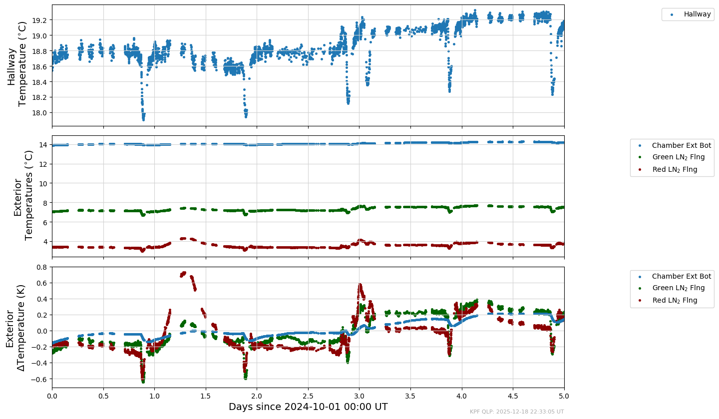
The AnalyzeTimeSeries has a built-in plotting library that uses dictionaries to describe the elements of plots. An example is shown below. Note that start_date and end_date are formatted as datetime objects, not strings as above.

[11]:

start_date = datetime(2024, 10,  1)
end_date   = datetime(2024, 10,  6)
dict1 = {'col': 'kpfmet.TEMP',              'plot_type': 'scatter', 'unit': 'K', 'plot_attr': {'label':  'Hallway',              'marker': '.', 'linewidth': 0.5}}
dict2 = {'col': 'kpfmet.GREEN_LN2_FLANGE',  'plot_type': 'scatter', 'unit': 'K', 'plot_attr': {'label': r'Green LN$_2$ Flng',    'marker': '.', 'linewidth': 0.5, 'color': 'darkgreen'}}
dict3 = {'col': 'kpfmet.RED_LN2_FLANGE',    'plot_type': 'scatter', 'unit': 'K', 'plot_attr': {'label': r'Red LN$_2$ Flng',      'marker': '.', 'linewidth': 0.5, 'color': 'darkred'}}
dict4 = {'col': 'kpfmet.CHAMBER_EXT_BOTTOM','plot_type': 'scatter', 'unit': 'K', 'plot_attr': {'label': r'Chamber Ext Bot',      'marker': '.', 'linewidth': 0.5}}
dict5 = {'col': 'kpfmet.CHAMBER_EXT_TOP',   'plot_type': 'plot',    'unit': 'K', 'plot_attr': {'label': r'Chamber Exterior Top', 'marker': '.', 'linewidth': 0.5}}
thispanelvars = [dict1]
thispaneldict = {'ylabel': 'Hallway\n' + r' Temperature ($^{\circ}$C)',
                 'legend_frac_size': 0.3}
halltemppanel = {'panelvars': thispanelvars,
                 'paneldict': thispaneldict}

thispanelvars2 = [dict2, dict3, dict4]
thispaneldict2 = {'ylabel': 'Exterior\n' + r' Temperatures ($^{\circ}$C)',
                 'legend_frac_size': 0.3}
halltemppanel2 = {'panelvars': thispanelvars2,
                  'paneldict': thispaneldict2}

thispanelvars3 = [dict2, dict3, dict4]
thispaneldict3 = {'ylabel': 'Exterior\n' + r'$\Delta$Temperature (K)',
                 'subtractmedian': 'true',
                 'legend_frac_size': 0.3}
halltemppanel3 = {'panelvars': thispanelvars3,
                  'paneldict': thispaneldict3}

panel_arr = [halltemppanel, halltemppanel2, halltemppanel3]

plotdict = {
             "description": "Etalon RVs (autocal)",
             "plot_type": "time_series_multipanel",
             "panel_arr": panel_arr
            }
myTS.plot_time_series_multipanel(plotdict, start_date=start_date, end_date=end_date, show_plot=True, clean=True)

../_images/tutorials_AnalyzeTimeSeries_Tutorial_27_0.png

The method plot_time_series_multipanel() above was written originally for use with dictionaries as shown above. However, it became easier to the plotting configuration in YAML files and convert to Python dictionaries when reading the configuration. An example of a configuration file is shown below.

[12]:

!cat /code/KPF-Pipeline/static/tsdb_plot_configs/QC/qc_lfc.yaml

description: QC - LFC Metrics
plot_type: time_series_multipanel
panel_arr:
  - panelvars:
      - col: LFCSAT
        plot_type: state
        plot_attr:
          label: LFC Not Saturated
          marker: .
    paneldict:
      ylabel: "LFC Not Saturated\n(LFCSAT)"
      legend_frac_size: 0.15
      only_object:
        - autocal-lfc-all-morn
        - autocal-lfc-all-eve
        - autocal-lfc-all-night
        - cal-LFC
        - cal-LFC-morn
        - cal-LFC-eve
        - LFC_all
        - lfc_all
        - LFC
      not_junk: true
      qc_not_fail: 'GOODREAD, FLXSTATS, DATAPRL0, KWRDPRL0, TIMCHKL0'

  - panelvars:
      - col: LFC2DFOK
        plot_type: state
        plot_attr:
          label: "2D LFC Flux Meets\nThreshold of 4000 Counts"
          marker: .
    paneldict:
      ylabel: "2D LFC Flux Meets Threshold\nof 4000 Counts\n(LFC2DFOK)"
      legend_frac_size: 0.15
      only_object:
        - autocal-lfc-all-morn
        - autocal-lfc-all-eve
        - autocal-lfc-all-night
        - cal-LFC
        - cal-LFC-morn
        - cal-LFC-eve
        - LFC_all
        - lfc_all
        - LFC
      not_junk: true
      qc_not_fail: 'GOODREAD, FLXSTATS, DATAPRL0, KWRDPRL0, TIMCHKL0'

  - panelvars:
      - col: LFCLINEP
        plot_type: state
        plot_attr:
          label: "Number and dist of\nLFC lines sufficient\n(SCI orders 15-34, 1-31)"
          marker: .
    paneldict:
      ylabel: "Number and dist of\nLFC lines sufficient\n(SCI orders 15-34, 1-31)\n(LFCLINEP)"
      legend_frac_size: 0.15
      only_object:
        - autocal-lfc-all-morn
        - autocal-lfc-all-eve
        - autocal-lfc-all-night
        - cal-LFC
        - cal-LFC-morn
        - cal-LFC-eve
        - LFC_all
        - lfc_all
        - LFC
      not_junk: true
      qc_not_fail: 'GOODREAD, FLXSTATS, DATAPRL0, KWRDPRL0, TIMCHKL0'

  - panelvars:
      - col: LFCLINES
        plot_type: state
        plot_attr:
          label: "Number and dist of\nLFC lines sufficient\n(SCI orders 2-34, 1-31)"
          marker: .
    paneldict:
      ylabel: "Number and dist of\nLFC lines sufficient\n(SCI orders 2-34, 1-31)\n(LFCLINES)"
      title: QC - LFC Metrics
      legend_frac_size: 0.15
      only_object:
        - autocal-lfc-all-morn
        - autocal-lfc-all-eve
        - autocal-lfc-all-night
        - cal-LFC
        - cal-LFC-morn
        - cal-LFC-eve
        - LFC_all
        - lfc_all
        - LFC
      not_junk: true
      qc_not_fail: 'GOODREAD, FLXSTATS, DATAPRL0, KWRDPRL0, TIMCHKL0'

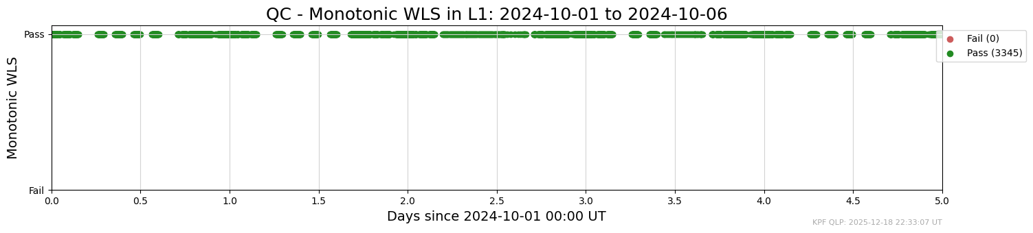
This simple example is equivalent to the dictionary plotdict below.

[13]:

dict1 = {'col': 'MONOTWLS',
         'plot_type': 'state',
         'plot_attr': {'label':'Montonic WLS','marker': '.'}}
thispanelvars = [dict1]
thispaneldict = {'ylabel': 'Montonic WLS',
                 'title': 'QC - Monotonic WLS in L1',
                 'legend_frac_size': 0.10}

lfcpanel = {'panelvars': thispanelvars,
            'paneldict': thispaneldict}

panel_arr = [lfcpanel]
mydict = {
    "description": "QC - Monotonic WLS in L1",
    "plot_type": "time_series_multipanel",
    "panel_arr": panel_arr
}

[14]:

myyaml = '''description: QC - Monotonic WLS in L1
plot_type: time_series_multipanel
panel_arr:
  - panelvars:
      - col: MONOTWLS
        plot_type: state
        plot_attr:
          label: Montonic WLS
          marker: .
    paneldict:
      ylabel: Monotonic WLS
      title: QC - Monotonic WLS in L1
      legend_frac_size: 0.10
'''

Below are plots of the dictionary and yaml representations.

[15]:

# Dictionary version
myTS.plot_time_series_multipanel(mydict, start_date=start_date, end_date=end_date, show_plot=True, clean=True)

# YAML version
myyaml_converted = myTS.yaml_to_dict(myyaml)
myTS.plot_time_series_multipanel(myyaml_converted, start_date=start_date, end_date=end_date, show_plot=True, clean=True)

../_images/tutorials_AnalyzeTimeSeries_Tutorial_34_0.png

../_images/tutorials_AnalyzeTimeSeries_Tutorial_34_1.png

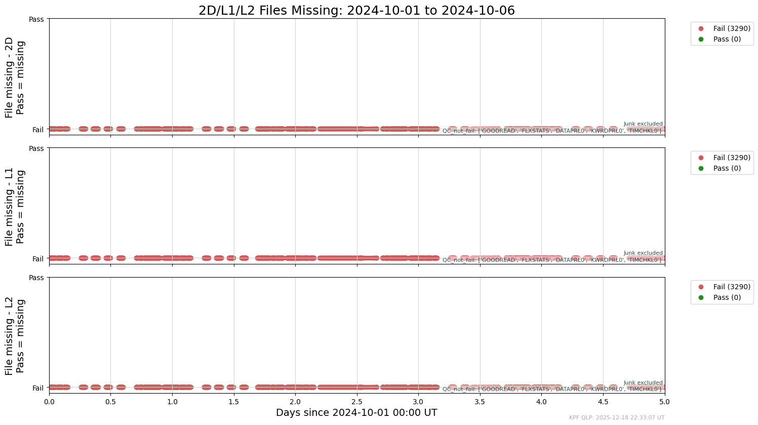
Plotting Telemetry

Examples of two built-in standard telemetry plots are shown below.

[16]:

myTS.plot_time_series_multipanel('files_missing', start_date=start_date, end_date=end_date, show_plot=True, clean=True)

INFO: Plotting from config: /code/KPF-Pipeline/static/tsdb_plot_configs/DRP/files_missing.yaml

../_images/tutorials_AnalyzeTimeSeries_Tutorial_36_1.png

[17]:

myTS.plot_time_series_multipanel('ccd_temp', start_date=start_date, end_date=end_date, show_plot=True, clean=True)

INFO: Plotting from config: /code/KPF-Pipeline/static/tsdb_plot_configs/CCDs/ccd_temp.yaml

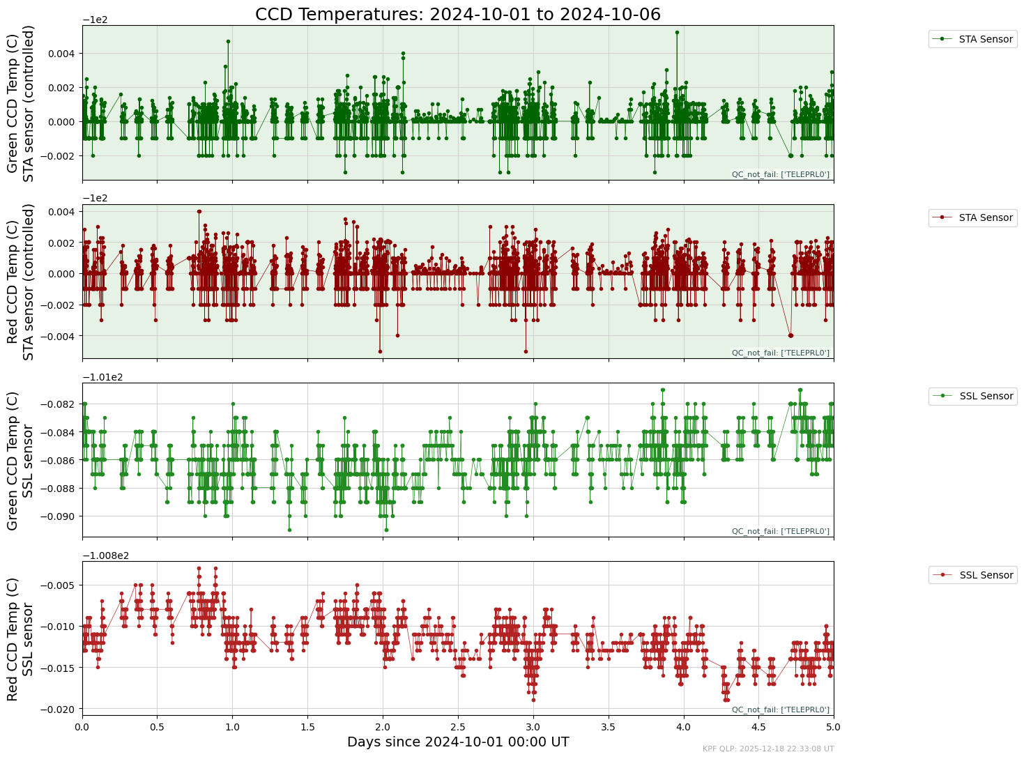
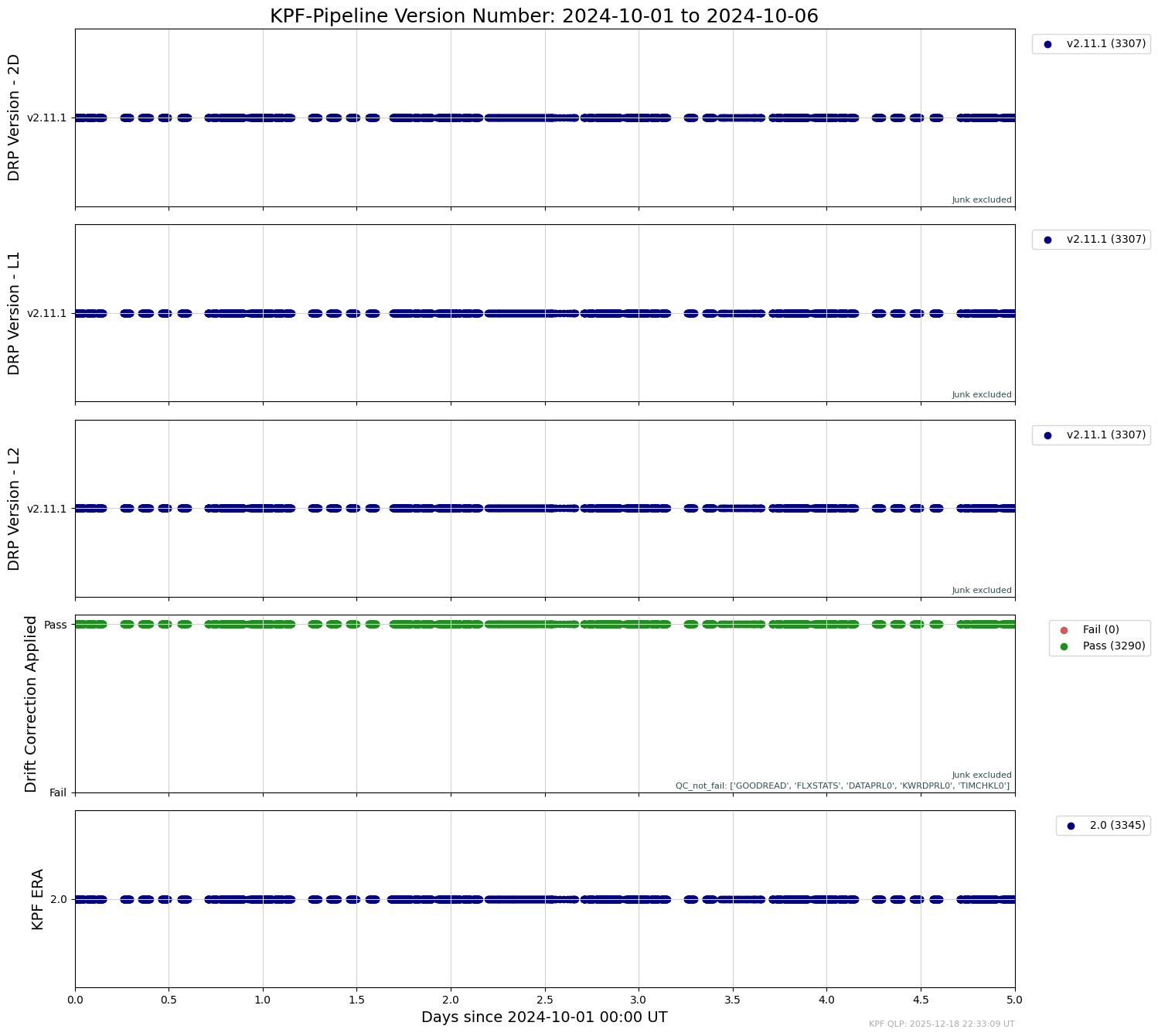
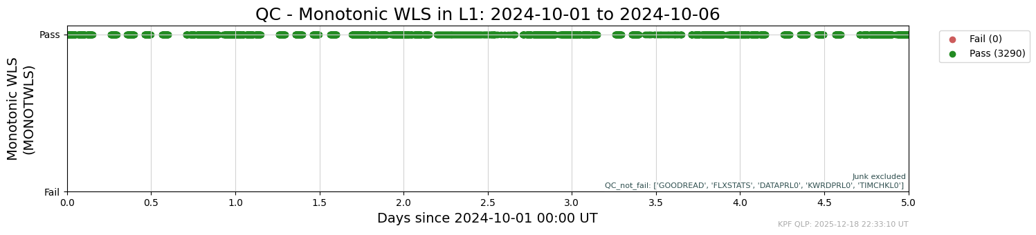
../_images/tutorials_AnalyzeTimeSeries_Tutorial_37_1.png

The examples above are all plots of float-type variables (e.g., temperatures) over time. The two below sho examples of state variables changing over time (the DRP version number used to process the data and the result of a quality control test).

[18]:

myTS.plot_time_series_multipanel('drptag', start_date=start_date, end_date=end_date, show_plot=True, clean=True)

INFO: Plotting from config: /code/KPF-Pipeline/static/tsdb_plot_configs/DRP/drptag.yaml

../_images/tutorials_AnalyzeTimeSeries_Tutorial_39_1.png

[19]:

myTS.plot_time_series_multipanel('qc_monotonic_wls', start_date=start_date, end_date=end_date, show_plot=True, clean=True)

INFO: Plotting from config: /code/KPF-Pipeline/static/tsdb_plot_configs/QC/qc_monotonic_wls.yaml

../_images/tutorials_AnalyzeTimeSeries_Tutorial_40_1.png

Plotting RVs

An example of plotting RVs (instead of telemetry) is shown below.

[20]:

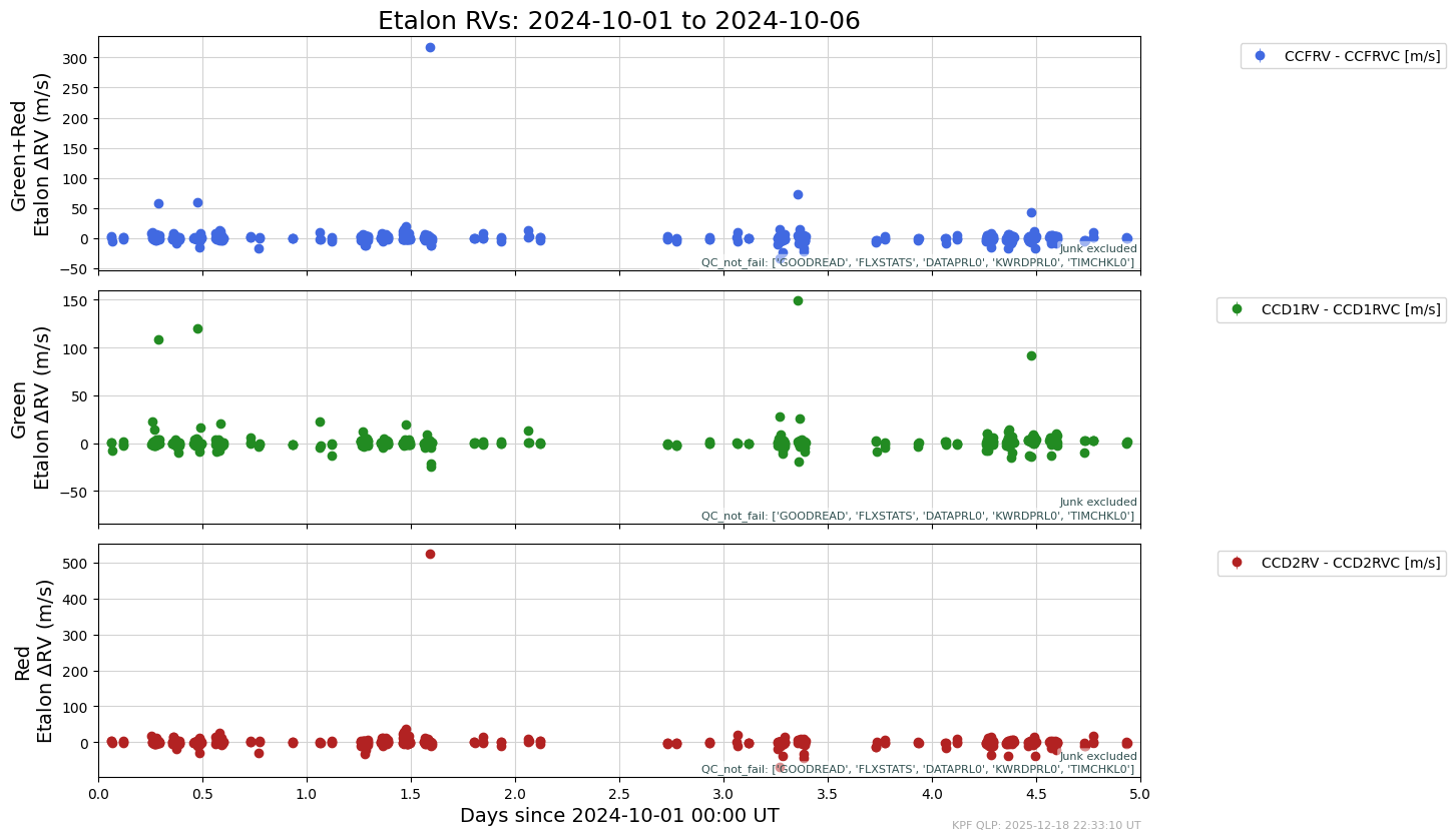
myTS.plot_time_series_multipanel('autocal_etalon_rv', start_date=start_date, end_date=end_date, show_plot=True, clean=True)

INFO: Plotting from config: /code/KPF-Pipeline/static/tsdb_plot_configs/RV/autocal_etalon_rv.yaml

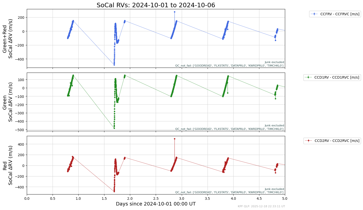
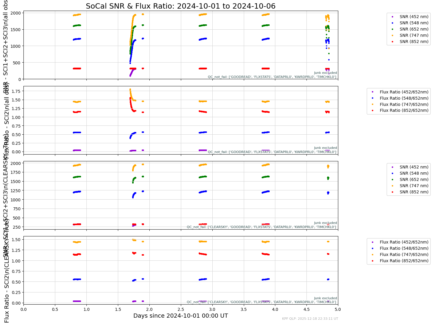
../_images/tutorials_AnalyzeTimeSeries_Tutorial_43_1.png

Here’s an example of plotting SoCal RV and spectral SNR time series.

[21]:

myTS.plot_time_series_multipanel('socal_rv',  start_date=start_date, end_date=end_date, show_plot=True, clean=True)
myTS.plot_time_series_multipanel('socal_snr', start_date=start_date, end_date=end_date, show_plot=True, clean=True)

INFO: Plotting from config: /code/KPF-Pipeline/static/tsdb_plot_configs/RV/socal_rv.yaml

../_images/tutorials_AnalyzeTimeSeries_Tutorial_45_1.png

INFO: Plotting from config: /code/KPF-Pipeline/static/tsdb_plot_configs/SoCal/socal_snr.yaml

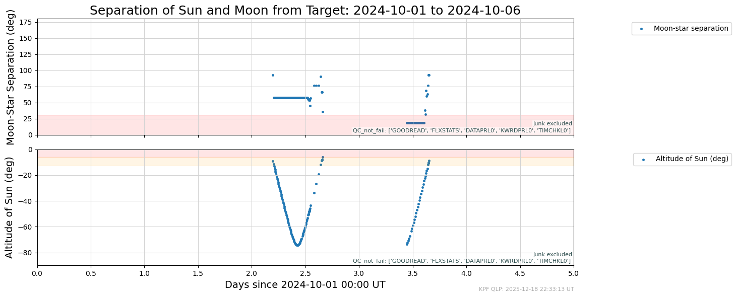
../_images/tutorials_AnalyzeTimeSeries_Tutorial_45_3.png

One can also plot information about on-sky conditions.

[22]:

myTS.plot_time_series_multipanel('seeing',   start_date=start_date, end_date=end_date, show_plot=True, clean=True)
myTS.plot_time_series_multipanel('sun_moon', start_date=start_date, end_date=end_date, show_plot=True, clean=True)

INFO: Plotting from config: /code/KPF-Pipeline/static/tsdb_plot_configs/Observing/seeing.yaml

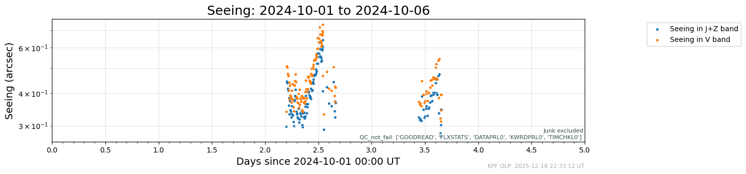
../_images/tutorials_AnalyzeTimeSeries_Tutorial_47_1.png

INFO: Plotting from config: /code/KPF-Pipeline/static/tsdb_plot_configs/Observing/sun_moon.yaml

../_images/tutorials_AnalyzeTimeSeries_Tutorial_47_3.png

Here’s the docstring describing the full set of options for AnalyzeTimeseries.plot_time_series_multipanel.

[23]:

myTS.plot_time_series_multipanel?

Signature:
myTS.plot_time_series_multipanel(
    plotdict,
    start_date=None,
    end_date=None,
    hatch_service_missions=True,
    clean=False,
    fig_path=None,
    show_plot=False,
    log_savefig_timing=False,
)
Docstring:
Generate a multi-panel time series plot from a KPF TSDB. Each subplot is configured
via a dict (or YAML file path), enabling control over filters, transforms, and style.

Parameters
----------
plotdict : str or dict
    Path to a named YAML config or a dict with key 'panel_arr' (list of panel dicts).
start_date, end_date : datetime, optional
    Query window (UT). Defaults if None: start=2020-01-01, end=2040-01-01. The code
    may tighten to the data’s min/max timestamps.
hatch_service_missions : bool, default=True
    Overlay hatched spans from self.get_service_mission_df() (UT_start_date, UT_end_date).
clean : bool, default=False
    Apply self.db.clean_df() to remove outliers.
fig_path : str, optional
    Full output path (PNG).
show_plot : bool, default=False
    Show the figure interactively.
log_savefig_timing : bool, default=False
    Log CPU time for savefig().

Plot Configuration (via panel_dict or YAML)
-------------------------------------------
plotdict['panel_arr'] : list[dict]
    Each element defines one panel and includes:

    - 'paneldict' : dict   # panel-level behavior/filters
        - 'only_object' : str | list[str]          # exact OBJECT names
        - 'object_like' : str | list[str]          # LIKE patterns (nested lists ok)
        - 'only_source' : str                      # passed to DB filter layer
        - 'not_junk' : bool | {'true','false'}     # filter on NOTJUNK
        - 'qc_pass' : str | list[str]              # columns that must be True
        - 'qc_fail' : str | list[str]              # columns that must be False
        - 'qc_not_pass' : str | list[str]          # columns that are not True (False/NaN)
        - 'qc_not_fail' : str | list[str]          # columns that are not False (True/NaN)
        - 'on_sky' : bool | {'true','false'}       # True→FIUMODE=='Observing', False→'Calibration'
        - 'ylabel' : str                           # label for vertical axis
        - 'ylim' : tuple | str                     # (ymin, ymax) or a string that evals to that
        - 'ymin', 'ymax' : float                   # override parts of ylim
        - 'yscale' : str                           # e.g., 'log'
        - 'subtractmedian' : bool                  # subtract per-variable median before plotting
        - 'nolegend' : bool                        # suppresses legend
        - 'labelrms' : bool                        # add legend text like ""(0.001 C rms)"
        - 'legend_frac_size' : float               # legend anchor offset
        - 'axhspan' : dict                         # {key: {'ymin','ymax','color','alpha'}}
        - 'title' : str                            # title for a set of panels
        - 'narrow_xlim_daily' : bool               # shrink x-limits to data for day-scale plots

    - 'panelvars' : list[dict]   # variables drawn in this panel
        - 'col' : str                                # main data column
        - 'col_err' : str                            # symmetric error column (optional)
        - 'col_subtract' : str                       # subtract this column from 'col'
        - 'col_multiply' : float                     # scalar multiplier
        - 'col_offset' : float                       # scalar offset
        - 'normalize' : bool                         # divide by median after transforms
        - 'plot_type' : {                            # determine plot type
             'scatter',                              # scatter plot (default)
             'errorbar',                             # errorbar plot; must include 'col_err'
             'plot',                                 # line plot
             'step',                                 # step plot
             'state',                                # state value plot with distinct values, usually strings or booleans
             'vlines'                                # plot with vertical lines; must include 'col_min' and 'col_max'
             }
        - 'plot_attr' : dict                         # matplotlib kwargs (marker, label, etc.)
        - 'unit' : str                               # used when augmenting legend label with RMS
        - 'col_min','col_max' : str                  # required for plot_type='vlines'
        - 'vline_pt_color' : str                     # optional color for vline end points

Returns
-------
None
    Saves to fig_path (if given), optionally shows, and logs as configured.

Notes
-----
- Time axis adapts to span:
    * ~1 day: hours since start (UT/HST labels possible), optional “Night” shading
    * <3 days or <32 days: days since start
    * 28–31 days: month view (day numbers)
    * ~1 year: month tick marks with MM-DD labels
    * longer: calendar dates (YYYY-MM-DD)
- 'state' plots render categorical levels; {0,1,None}→{Fail,Pass,None}. If ylabel=='Junk Status',
  {Pass,Fail}→{Not Junk,Junk}.
- Empty selections are annotated “No Data”.
- Labels may be augmented with “(X unit rms)” when legend shown and enough points exist.
- Data come from self.db.dataframe_from_db(...); DATE-MID parsed and sorted; clean_df() optional.
File:      /code/KPF-Pipeline/modules/quicklook/src/analyze_time_series.py
Type:      method

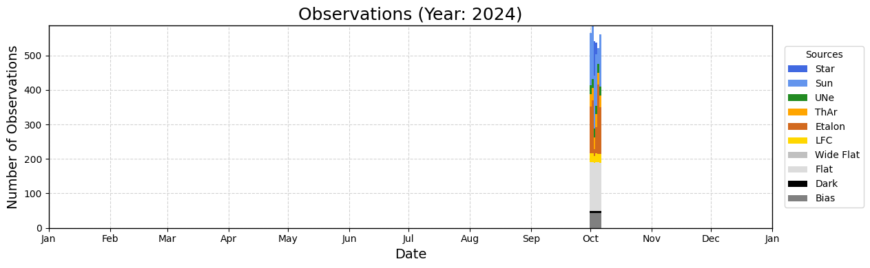
Making Histograms of the Number Observations Over Time

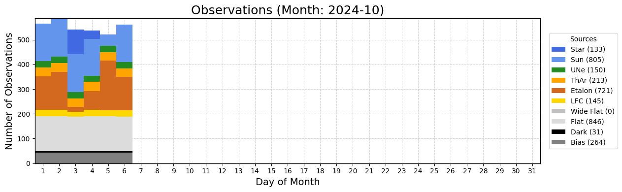
Make a plot of the number of observations for the whole time span that’s been ingested.

[24]:

myTS.plot_nobs_histogram(interval='year', date='20241002', show_plot=True, plot_source=True)

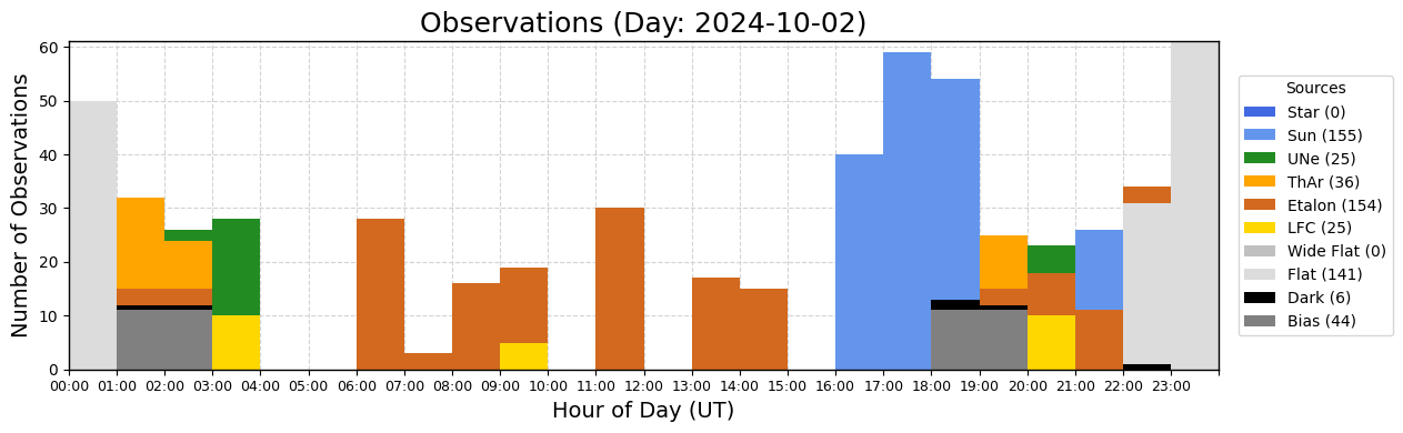
../_images/tutorials_AnalyzeTimeSeries_Tutorial_52_0.png

Show the observations by type for the that month and one day.

[25]:

myTS.plot_nobs_histogram(interval='month', date='20241002', plot_source=True, show_plot=True)

../_images/tutorials_AnalyzeTimeSeries_Tutorial_54_0.png

[26]:

myTS.plot_nobs_histogram(interval='day', date='20241002', plot_source=True, show_plot=True)

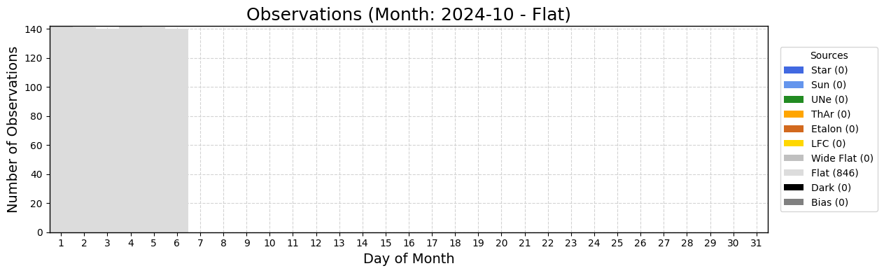
../_images/tutorials_AnalyzeTimeSeries_Tutorial_55_0.png

Show the number of observations of just one source over a month.

[27]:

myTS.plot_nobs_histogram(interval='month', date='20241002', plot_source=True, show_plot=True, only_sources=['Flat'])

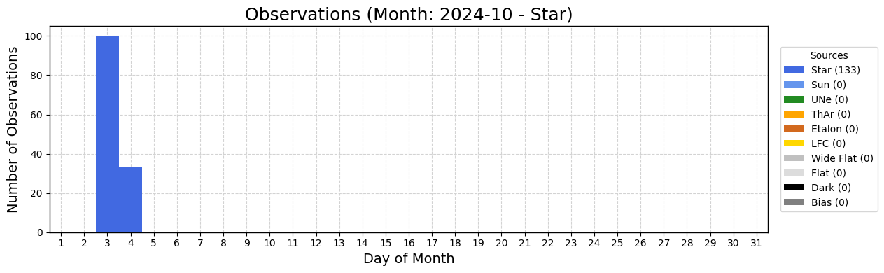
../_images/tutorials_AnalyzeTimeSeries_Tutorial_57_0.png

Show the number of stell observations per UT night.

[28]:

myTS.plot_nobs_histogram(interval='month', date='20241002', plot_source=True, show_plot=True, only_sources=['Star'])

../_images/tutorials_AnalyzeTimeSeries_Tutorial_59_0.png

The Full Set of Standard Plots

There are also a number of standard plots based on YAML files in subdirectories of KPF-Pipeline/static/tsdb_plot_configs/. The full set is listed below.

[29]:

myTS.plot_all_quicklook(print_plot_names=True)

Plots available:
    'ccd_controller': CCD Controller Temperatures
    'ccd_dark_current': CCD Dark Current
    'ccd_readnoise': CCD Read Noise
    'ccd_readspeed': CCD Read Speed
    'ccd_temp': CCD Temperatures
    'ccd_noise_stats': CCD Read Noise Statistics
    'xdisp_offset': CCD Cross Dispersion Offsets
    'ccd_pressure': CCD Pressures
    'saturated_etalon': Saturated Lines - Etalon
    'saturated_thar': Saturated Lines - ThAr
    'autocal-flat_flux_relative': autocal-flat-all Relative Flux Ratio
    'autocal-flat_snr': autocal-flat-all SNR & Flux Ratio
    'autocal-flat_snr_relative': autocal-flat-all Relative SNR Ratio
    'good_orders_etalon': Good Orders - Etalon
    'good_orders_lfc': Good Orders - LFC
    'hcl': Hollow-Cathode Lamp Temperatures
    'lamp_power': Power Meter Measurements of Lamp Brightness
    'last_good_cal': Last Good LFC and Etalon Calibrations
    'saturated_lfc': Saturated Lines - LFC
    'lfc_freq': LFC Diagnostics
    'autocal-etalon_snr': autocal-etalon and slewcal SNR
    'lfc': LFC Diagnostics
    'autocal-etalon_flux_ratio': autocal-etalon Flux Ratios
    'saturated_une': Saturated Lines - Une
    'chamber_temp': KPF Spectrometer Temperatures
    'chamber_temp_detail': Chamber Temperature Detail
    'hallway_temp': KPF Hallway Temperature
    'spatial_gradients': KPF Spectrometer Spatial Temperature Gradients
    'drphash': KPF-Pipeline Commit Hash
    'drptag': KPF-Pipeline Version Number
    'files_missing': 2D/L1/L2 Files Missing
    'master_age': Ages of Master Files
    'nobs_all_sources': All Sources - Number of Observations
    'nobs_bias': Bias autocal - Number of Observations
    'nobs_dark': Dark autocal - Number of Observations
    'nobs_flat': Flat autocal - Number of Observations
    'nobs_lfc': LFC autocal - Number of Observations
    'nobs_sun': SoCal - Number of Observations
    'nobs_all_good_sources': All Sources - Number of Observations
    'nobs_star': Stars - Number of Observations
    'bcvel': Barycentric Variations
    'guider_images': Guider Images
    'guiding': Guiding Errors & Bias
    'observing_snr': Observing SNR & Flux Ratio for Stars
    'seeing': Seeing
    'sun_moon': Separation of Sun and Moon from Target
    'junk_status': Junk Status and Smeared Readout Assessment
    'qc_agitator': QC - Agitator Running
    'qc_cals': QC - Flat SNR
    'qc_ccd_temp': QC - CCD Temperature Set Points
    'qc_data_kwds': QC - Data and Keywords Present
    'qc_em': QC - Exposure Meter
    'qc_etalon': QC - Etalon Metrics
    'qc_flat': QC - Flat Metrics
    'qc_guider': QC - Guider Performance
    'qc_hk': QC - CaHK Shutter
    'qc_kwds': QC - TARG Keywords
    'qc_lfc': QC - LFC Metrics
    'qc_low_flux': QC - Low Dark and Bias Flux
    'qc_master_age': QC - Master File Ages
    'qc_monotonic_wls': QC - Monotonic WLS in L1
    'qc_ntp': QC - Network Time Protocol (NTP)
    'qc_observing': QC - Observing
    'qc_pos_2d_snr': QC - Not Negative 2D SNR
    'qc_time_check': QC - L0 and L2 Times Consistent
    'qc_wls': QC - Wavelength Solution Metrics
    'autocal_etalon_rv': Etalon RVs (autocal)
    'autocal_rv': LFC, ThAr, & Etalon RVs (autocal)
    'socal_rv': SoCal RVs
    'autocal_erv': LFC, ThAr, & Etalon ERVs (autocal)
    'clearsky': Seeing
    'socal_snr': SoCal SNR & Flux Ratio
    'wls_median': WLS Median Difference
    'wls_stdev': WLS Standard Deviation of (L1 - L1_ref)
    'agitator': KPF Agitator
    'fiber_temp': Fiber Temperatures
    'hk_temp': Ca H&K Spectrometer Temperatures
    'etalon': Etalon Temperatures

Generating All Standard Plots

One can also generate all plots from the plot_all_quicklook_daterange() method with a single call. It is in an if statement below so that be disabled because it generates a large number of plots (a few dozen) that may be more than are desired. Toggle if False: to if True: to show the output.

[30]:

if False:
    myTS = AnalyzeTimeSeries(db_path=db_path)
    myTS.plot_all_quicklook(datetime(2024, 10, 3), interval='day', show_plot=True, verbose=True)